In the original transformer architecture, Vaswani et al. introduced sinusoidal positional encodings, given by
PE(pos,2i)=sin(pos/100002i/dmodel)
PE(pos,2i+1)=cos(pos/100002i/dmodel)
In their words:
We chose [sinusoidal encoding] because we hypothesized it would allow the model to easily
learn to attend by relative positions, since for any fixed offset k, PEpos+k can be
represented as a linear function of PEpos. (Vaswani et al.)
To see the linearity, first write (by the trigonometric angle sum identities)
PE(pos+k,2i)=sin((pos+k)/100002i/dmodel)=PE(pos,2i)PE(k,2i+1)+PE(k,2i)PE(pos,2i+1)
for the even dimensions and
PE(pos+k,2i+1)=cos((pos+k)/100002i/dmodel)=PE(pos,2i+1)PE(k,2i+1)−PE(k,2i)PE(pos,2i)
for the odd ones. Now note that
PEpos+k:=[PE(pos+k,2i)PE(pos+k,2i+1)]
=[PE(k,2i+1)−PE(k,2i)PE(k,2i)PE(k,2i+1)][PE(pos,2i)PE(pos,2i+1)],
which is a rotation of PEpos.
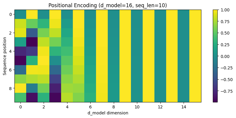
However, I prefer to emphasize the fact that sinusoidal encodings capture both long-range and short-range dependencies. Consider the following heatmap, which plots PE (color) against dimension and sequence position:

For small i, the period of the sinusoidal functions is minimized, leading to greater variation among nearby tokens. Note that in the leftmost column, highly variable colors cluster together.
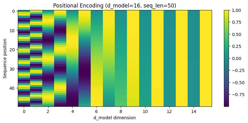
But a small period makes it harder to distinguish between distant positions. Say we increase the sequence length to 50:

While dimension 0 assigns identical values to positions 0 and 41, among others, dimensions 4-7 (which have lower frequency) clearly differentiate between them.

